A detailed explanation of the 10,000-character record BEV perception scheme and deployment practice based on Journey 5

Introduction:

On August 24th, the latest issue of Horizon’s "Hello, Developer" Autopilot Technology Special Session was successfully broadcast in the Zhidong Open Class.

The special session was given by Dr. algorithm engineer Zhu Hongmei, Horizon Perception, with the theme of BEV Perception Scheme and Deployment Practice Based on Journey 5. This article is a record of the lecture session of this special session. If you need live playback and Q&A, you can click

Good evening, friends of the open class of Zhidong. I’m Perception algorithm engineer Zhu Hongmei from the horizon, and I’m honored to share with you today "Ji"BEV awareness scheme and deployment practice in Journey 5》。 I will introduce it from five aspects.

01

General introduction of BEV perception framework

With the release of Journey 5 in 2021, we designed the sensing prototype scheme of BEV based on Journey 5. The input is vehicle-mounted multi-angle image sequence or multi-mode signal, and the fusion of time and space dimensions is carried out within the network, so that the neural network can output the dynamic and static sensing and prediction results from a bird’s-eye view.

Below is a frame diagram.

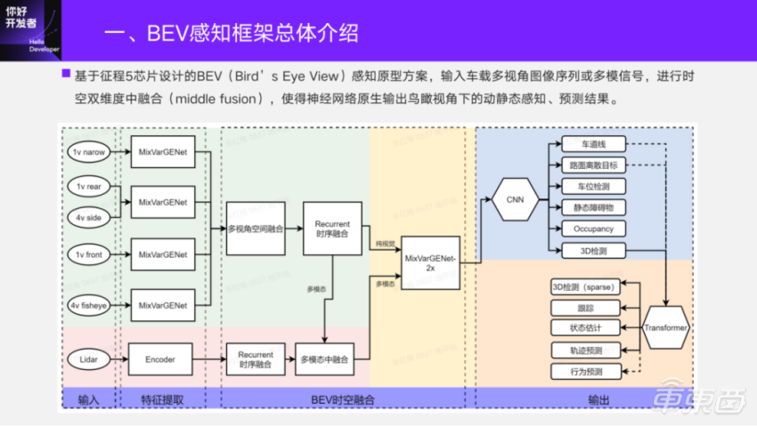
The green background part represents the signal processing of pure vision, and the input is the images of each camera. After the first stage of model extraction, the image features are transformed into multi-view spatial fusion from BEV perspective. Then, the features of BEV are fused in time sequence, and then sent to the second stage for feature extraction on BEV; Finally, input it to the head part for the output of perceptual elements. If there is a Lidar in the system, it will also be connected to the Lidar point cloud. In the early stage, we will do rasterization coding processing, and we will also do time sequence fusion. Finally, we will do intermediate fusion with visual BEV features, and also send them to the second stage to output the perceptual elements on BEV.

The blue part is the closed-loop iteration that has participated in many rounds. Students who pay attention to the horizon should know that at the Shanghai Auto Show in April this year, this part of the content has supported the closed-loop demo display of real cars. In recent six months, we have expanded the function of "dynamic obstacle detection" in sensing elements. Based on it, we connected the head of Transformer to do the Track id, speed estimation and trajectory prediction of dynamic obstacles. The dotted line part is currently under development, and we also want to make full use of the dynamic and static sensing results on BEV to output the interactive elements of dynamic and static sensing, such as behavior prediction.

There are two main modes of pure vision scheme here. One is the 11v integration scheme for double Journey 5; The other is a single journey chip-oriented scheme, in which 7v for driving and 5v for parking are integrated. Today’s sharing mainly focuses on the integration of time and space in the visual scheme, the analysis of perceptual elements, and the introduction of dynamic, especially dynamic perceptual prediction end-to-end scheme and deployment.

02

Spatio-temporal fusion module and chip deployment

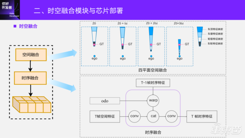
Firstly, it is introduced that the four-plane space fusion method is adopted at the end of the plate at present. It takes the xy plane of the self-propelled coordinate system as the basic plane, and adds three height planes on this basis, hoping to obtain more scene image information with different heights. Time series fusion is relatively simple. We will cache the features after time series fusion at the last moment, align the historical frames to the current frame by using the self-driving motion between frames, and fuse them with the spatial fusion features of the current frame, and then deconvolution them and send them to the following network structure for perceptual output.

So why do we use this scheme?

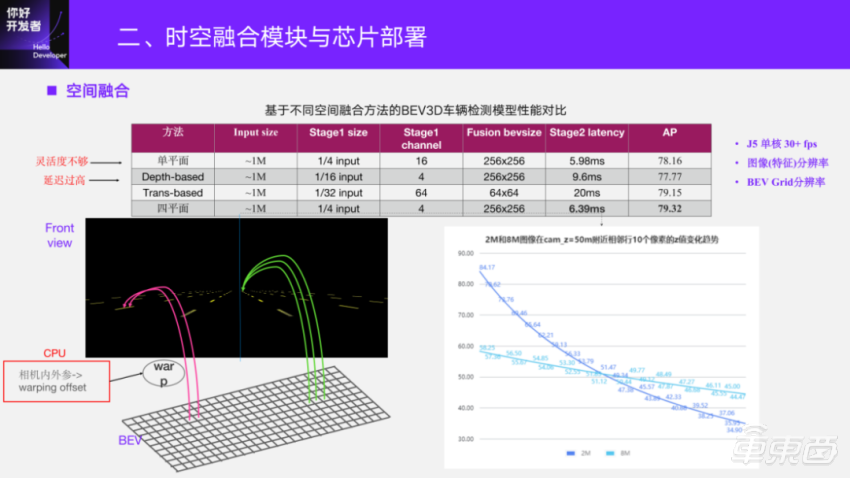
In the early stage of research and development, we also compared different spatial fusion methods. In the early stage, in order to quickly get through the process, we adopted the simplest method based on single plane IPM to get through the perception of the whole framework. After that, I went to find out the depth-based fusion and transformer-based fusion scheme on Journey 5. The assessment dimension is the delay in Journey 5, assuming that the prerequisite is to be able to independently run this model above 30fps on the single core of Journey 5 to design the corresponding network parameters.

There are two key parameters that affect the perceptual performance of BEV, one is the resolution of image feature in one stage, and the other is the fusion resolution on BEV. The fusion resolution on BEV is relatively direct, and the higher the resolution, the better the perception of some small targets and point elements. Image resolution determines the amount of information input in two stages.

Here is a lane line simulation diagram, and the physical dimensions of each lane line are the same. Because it is perspective projection, the farther the lane line is in the image, the fewer pixels it will have. BEV indexing image features is generally a process of reverse realization, while BEV is generally designed with equal resolution, such as 0.6 and 0.4 m Grid resolution. When the distant objects in the scene are indexed by the coordinates of BEV, the physical resolution of the pixels in the image is already lower than that on BEV, and at this time, feature duplication will appear on BEV, which is a common stretching phenomenon. Reflected in the perception, for example, the detection box may have the phenomenon that the target splits into a string, so the feature resolution in one stage is also very important.

We grab the middle column of pixels to simulate the contrast of Z-value changes between two adjacent rows of pixels in 2M image and 8M image at 50m. It can be seen that the physical range of the low-resolution image corresponding to two adjacent rows of pixels has changed by more than 2 meters. For a high-resolution image, its adjacent two pixels are only about 0.6 meters. Therefore, when looking at the fusion scheme, we should not only consider whether a single task meets certain accuracy requirements, but also consider the final deployment, because it is multi-task and different perceptual elements output, so we hope that the resolution of one-stage feature and BEV fusion can be higher.

From this point of view, the current structure based on Transformer can meet the requirements of Journey 5, single core and 30+FPS, and the first-stage resolution and the second-stage fusion resolution are relatively low, and the delay is too high under this condition. However, the depth-based fusion method is lower than single plane in one stage. In addition, one reason for not adopting it is that the depth-based deployment has made some specific improvements for Journey 5, reaching a two-phase delay of 9.6 ms. In the stage of prototype verification, the flexibility of carrying different numbers of cameras on the car is not enough, so we adopt the plane mapping fusion method at this stage. In the early stage, we used a single plane, but when we actually did the closed-loop verification, we found that the generality and robustness of camera parameters were not enough, and it was sensitive. Therefore, we improved it in the further research and development process. Through various tests and verifications, we finally adopted the four-plane fusion method, which can achieve a good balance between performance and delay.

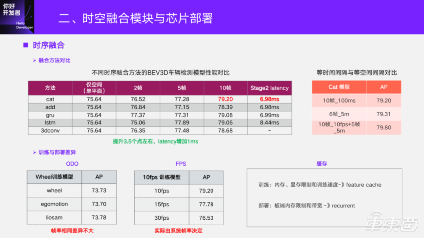
For time series fusion, different time series fusion methods will also be compared in the early stage of research and development. The basic method is to align the historical BEV features to the current frame and use different fusion methods to do time series fusion. Here is also a comparison of the fusion of different frames, with the experimental data accumulated at that time to do 10 frames of verification. In the case of 10 frames, there is an improvement of 3.5 points compared with only space. For latency, it is only increased by 1ms because it is deployed in recurrent mode.

Similarly, we also compare the two methods of obtaining historical frames. One is to intercept historical information at equal time intervals, and the other is at equal space intervals. Equal time interval is to use the system timestamp to index and read the corresponding frame. Equal space interval is to calculate the translation distance with the movement of the vehicle, and then get the frame. Finally, we found that the performance of equal space interval of 6 frames is similar to that of equal time interval of 10 frames, and they can also be combined, but the improvement of more fused frames is not great. Therefore, in order to simplify the deployment, we currently adopt the time series fusion method with equal time intervals.

There may be some differences in the training and deployment of time series fusion. One is the Odometry used when aligning two adjacent frames. In order to make the training model performance consistent with the real vehicle deployment, one principle to be observed is that the model input should be consistent with the board signal as much as possible. We use Odometry of wheel speedometer to do model training, and do tests on Odometry obtained by different methods. It is found that if it is consistent with the inter-frame interval during training, then this factor has little influence. In addition, for example, historical frames are obtained at 100ms intervals, and the model trained with 10fps training data is tested at 10fps, 15fps and 30fps. The conclusion is that if there is a big difference between deployment and training, the index gap will be even bigger. The actual system frame rate is affected by the real-time load of the system, and it may not be completely aligned no matter how to set the inter-frame interval during training. Generally, the perimeter perception can be around 15fps, which can basically meet the functional requirements, and the range of 1.5 points is also acceptable. This part can also make the distribution of time series training data more abundant through some data enhancement methods, and alleviate such problems.

The other is that when the time series is being trained, if there is no specific optimization, with the increase of the number of frames, some OOM(Out of Memorry) problems may occur in the time series data, which leads to the slow training speed. The training method is to adopt the feature cache strategy to alleviate or avoid such problems. However, when deploying on the board side, considering the memory limitation of the board side and the bandwidth loaded back, the most streamlined strategy recurrent mode is finally adopted on the board.

03

Analysis of static and Occupancy perception elements

An important component of static perception is truth value. How did the truth value on BEV come from?

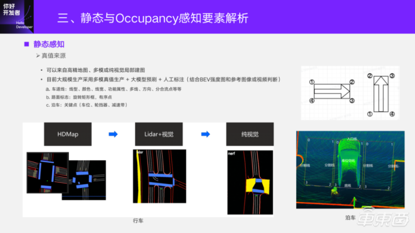
From the very beginning of research and development to the present, three static truth values have been used. At first, high-precision maps were used, and now the truth production link based on multi-mode is used on a large scale. At present, the local mapping results of pure vision are also involved in the training. The quality of the drawings is developed by our company’s special 4D-Label team. At the special session of horizon "Hello, developer" autopilot technology, Dr. Sui Wei, the head of horizon 4D labeling technology, also shared the "4D labeling scheme for BEV perception". If you are interested, you can review it.

For the algorithm, the algorithm students should be more involved in the formulation of labeling rules. Even if the truth value is brushed by the big model, the big model needs the truth value, so the labeling rules need the deep participation of the students of the perceptual algorithm, especially the actual test scenario is very complicated. A reference condition of labeling rules is the Lidar point cloud base map obtained by mapping, which is an intensity map on BEV, and then it can be labeled by referring to images or videos. For example, lane lines should be marked with colors, some functional attributes and some downstream functions that are necessary and cannot be obtained from the Lidar bottom map, all of which need to be combined with images. For pavement signs, they are usually unmarked rotating frames, and for those that need a clear direction, they need to be marked in an orderly sequence. The elements of parking are basically to mark parking spaces, wheel gears, speed bumps and so on by marking key points.

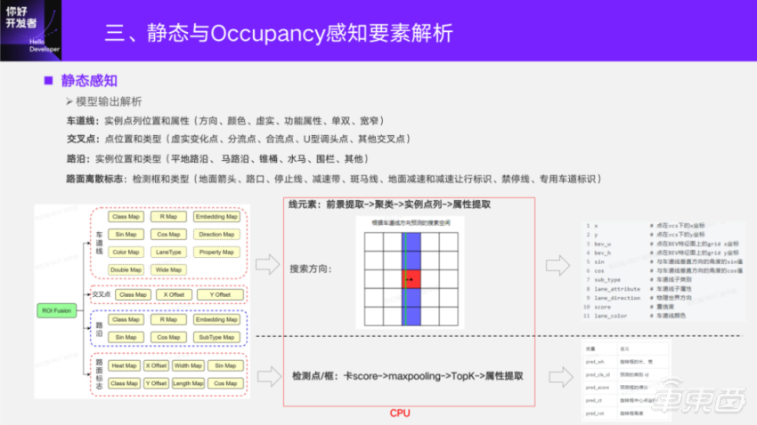
The output of the model corresponds to the annotation. The marked information will be preprocessed to generate the true value of the model. Only when the truth value is supervised output can the downstream functional requirements be met. The lane line output is the position and attribute of the example point column; The intersection point is the position and type of the point; Curbside is also the instance position and type; Pavement discrete signs are detection frames and types. These static perception elements are very rich. For the model scheme, there is a classification learning of foreground extraction, a regression learning of accurate position, and a learning of example features of lane lines. On the whole, the static perception scheme is relatively conventional. When analyzing, line elements such as lane lines will extract the foreground through the score of Class Map, then cluster the points through the Embedding similarity, and reverse the attribute features to index the corresponding features of these points.

For lane lines, in the actual software analysis, we should consider the delay on the software, roughly estimate the direction of lane lines through vertical points according to the preset, and do one-dimensional search along this direction to shorten the post-processing time of lane lines. Now our scheme is newly optimized, and it takes less than 3ms to deal with this part. The analysis of pavement signs, detection points or boxes at intersections is a set of CenterNet: card score→maxpolling→TopK→ attribute extraction → output.

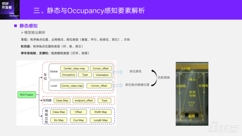
For parking elements, parking spaces will output orderly corner position, occupancy and parking space type direction; The wheel stopper is an orderly end position and type; The underground locks and columns under the parking lot are all output by detection frames, which are the same as the analytical ideas of the previous points and line frames. The parking space here has two small head, one of which is to obtain the overall attributes of the parking space, such as its occupancy, and whether the parking space type is parallel or vertical. There is also a Local head to accurately estimate the corner of the location, because the accuracy of this corner of the location is very high. After getting a more accurate one, calculate the point matching with the rough corner position obtained under global. Because this point is orderly, you can just card a distance threshold. After matching, you can get an accurate corner coordinate by replacing the corner coordinate.

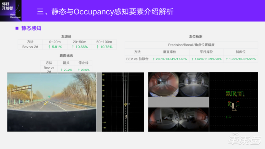
This is our performance. The 2D perception scheme of horizon has been polished for a long time before, which is equivalent to having a good reference baseline for BEV perception.

Compared with the 2D scheme, lane lines and road signs have a great improvement in ranging, such as lane lines in different distance sections, arrows and stop lines of road signs. For parking spaces, Horizon also has a pre-fusion scheme. Before being sent to the network, four fish-eye images are fused by IPM to get an IPM image covering 360 degrees around the car, and then integrated into the network to output parking spaces. Now BEV is introduced in the previous framework, and feature are fused inside the model. At present, there are also great improvements in these three class libraries.

Take a look at this video, which is a visual display of a high-speed lane line, with a wide dotted line, and then get off the ramp. Here is a diversion point, a change point between reality and reality, and the arrow represents the direction.

For the perception of parking space, a parking scene is chosen here, where the red line represents the entrance line, the yellow X represents the occupation, the yellow box is the pillar of the parking lot, and the grass green is the wheel stopper.

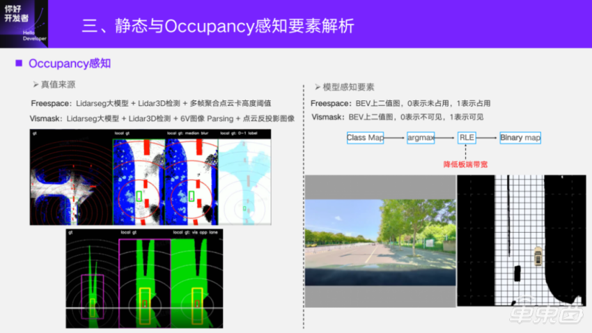
Let’s talk about the perception of Occupancy. First of all, Occupancy is a 2D occupancy graph based on Journey 5, which is a binary graph, where 0 means unoccupied and 1 means occupied. We call it Freespace internally. The traditional Freespace is image segmentation and post-processing to calculate the drivable area under BEV. It is more natural to do it on BEV, and output such a binary image directly on BEV. Its true value depends on Lidar segmentation model+detection model+threshold of cloud card height of multi-frame aggregation point to obtain some obstacles on the ground. Lidarseg mainly obtains the basic surface first, and takes the road plane as the drivable area; Lidar3D detection is to supplement the true value of dynamic obstacles in the white list.

The other output is Vismask. It mainly describes the area that the vehicle can see in the image at the current moment, and also uses Lidarseg model and 3D detection model. Image segmentation combined with back projection of point cloud can get the points that can be seen under BEV, calculate the ray according to the semantics and camera parameters, and then calculate the surface paved by the points that can be seen in the image in the self-propelled coordinate system, and then flatten them in the height direction of point cloud to get the visible Grid points on BEV. Why do you need 3D detection? Because when the ray hits the point cloud, it is a surface. We want the whole object of the surface boundary to be visible, so we need a 3D detection frame to supplement the object of the boundary, thus obtaining the true values of these two tasks. Perception model is a relatively simple binary classification model. Vismask’s 0 means invisible and 1 means visible.

Because these two tasks are dense outputs, when actually doing this on the board, its bandwidth occupation is relatively large. Usually, we will use a Run Length Encoding (RLE) to compress the result. For example, Freespace, as shown in the following figure, has the same values in a connected region. Run-length coding is used to reduce the bandwidth of the perceptual results transmitted from BPU of Journey 5 to CPU, and a final output binary image can be obtained by doing a back analysis in CPU.

Here is a visual video, and the bar on the left is a response to the fence. This is a specially built evaluation set, including strollers, fallen cones and so on. Here, Freespace is mainly to supplement the perception of non-standard obstacles. In addition, it is also useful to feed back the representation of roadside by Freespace when the downstream closed loop is used.

04

Dynamic Perception Predicting End-to-End and Chip Deployment

Let’s introduce the end-to-end scheme of dynamic sensing prediction and chip deployment.

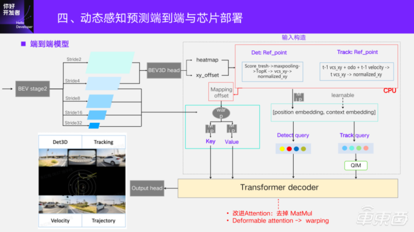
The end-to-end model, as shown in the previous frame, is followed BEV3D several layers of Transformer decoder to output dynamic end-to-end elements. The multi-scale features extracted by BEV in two stages are reused, and there is a detection head of BEV3D, which regresses to the heatmap and the offset to the precise position to get the possible target position.

For Transformer head, it depends on how the Q/K/V of its input comes from the first layer. There is a construction part of the input. First of all, "q" is divided into detection query and Track query. Detect the position embedding； of query, which is the position parsed from BEV3D head and obtained by MLP; Context embedding is learnable and can be initialized randomly.

For the position embedding of Track query, the position of the previous frame will be used, and the self-vehicle motion between frames will be aligned to the current frame to eliminate the self-vehicle motion. Then, the position of the current frame is estimated by combining the speed estimation result of the previous frame itself, and the position embedding of Track query is obtained by MLP. Its context embedding was also randomly initialized and learnable at the beginning, which resulted in "Q".

"K" and "V" For BEV, there is a fixed mapping relationship between the pixel coordinates on BEV and the coordinate positions under VCS. Therefore, according to the position of the reference point, its pixel coordinates on multiple dimensions of BEV can be calculated reversely. Query also sorts from 0 to N-1, and it has an index, so that the difference between the two coordinates can be calculated into the mapping relationship between them. Then the warping operator, that is, the grid_sample operator, is used to reversely index the BEV region features, and then "K" and "V" are generated through MLP, so that the end-to-end head input is constructed.

One of the differences in Transformer here is that it improves the quantization and efficiency on Journey 5, and removes the MatMul matrix multiplication operator. Here, the commonly used Deformable attention is replaced by warping.

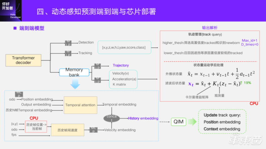
The output layer of end-to-end head is actually several MLPs. Among them, the output of trajectory and speed will pass through Memory bank in order to obtain historical information. The point of the trajectory output here is also the displacement between frames, and the velocity describes the position change of unit time between frames in the future. We think that these changes are not abrupt, but smooth, so we use historical information.

The embedding of history is composed of two parts. The first part is the Oddity of N historical frames and the embedding of query output by Transformer decoder of N historical frames will be stored in Memory bank. Query of the current frame, and pay attention to the time sequence of the current frame and the historical frame for each target. After that, self-attention will also be done among the targets, and finally we define it as Temporal embedding. In addition, speed embedding is added. How did it come from? That is, the position of historical frame N is transferred to the current frame through the odometry of the vehicle motion, and the position of the historical frame under the current frame is obtained, so as to eliminate the vehicle motion and obtain the inter-frame offset. Combining with the frame rate of the system, a time difference can be derived, and the historical inter-frame speed can be estimated. Similarly, after passing an MLP, the embedding of the speed can be obtained. By making a simple concat, the final historical embedding can be obtained and input to the trajectory.

After the model is output, some of it will be analyzed in CPU. For Track query and Detect query, the model output itself will analyze the position, length, width, height, orientation angle, Score confidence and so on. The function of track management is to screen out the Track query of the next frame. Two thresholds are set here. A higher threshold is to filter out the tracked query with higher confidence from all the queries, that is, the tracked query, and identify the newly generated target in the current frame. For the newly generated target, a current maximum id value of +1 is given, and its disappearance time is initialized to 0. For setting a low threshold, I want to recall those targets that have been tracked before, but have low confidence in the current frame due to occlusion and other reasons. If it can be greater than this threshold, and the disappearance time is not greater than the set time, it will continue to be preserved. If the time of disappearance (disp_times) has been greater than the threshold of the number of frames that can be dropped, we will definitely drop this target in this frame.

For the analysis of velocity, the model itself can be directly output, and kinematics post-processing will be added after it comes out. The "z" here is the length, width, height and speed (attribute) of the previous output, which we call observation. The model will also learn from the gain matrix of Kalman, avoiding calculating "k" on CPU, and finally giving the filtered state quantity to the downstream. Compared with the unfiltered operation, this operation has a 19% improvement in speed accuracy. From the visual performance, the speed does appear smoother after this. When updating the embedding of Track query in the next frame, the historical embedding generated in Memory bank will be used. The details of QIM will not be expanded, so you can refer to the implementation of MOTR.

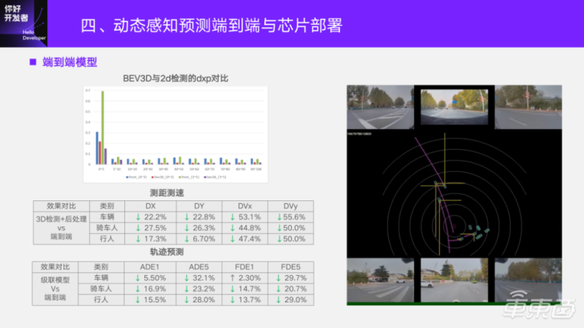
Take a closer look at the performance of the end-to-end model. End-to-end comparison is only detection, tracking and speed estimation through post-processing. The baseline detection compared here is already 3D detection on BEV. Compared with the original 2D detection, it has obvious advantages in ranging. Blue and green are the vertical error percentages of 2D detection in different distance segments, and red and purple are BEV3D. It can be seen that the end-to-end model is more advantageous than BEV3D on the basis of this better baseline.

First of all, take a look at ranging and speed measurement. From end to end, ranging and velocity measurement have obvious advantages on three kinds of dynamic obstacles. The lower the error here, the better, and here is the percentage of error reduction, especially the speed advantage is particularly obvious. Trajectory comparison is a cascade model, its input is the dynamic post-processing of 3D detection on BEV, and some vector information of lane line static post-processing after environmental reconstruction, which is a separate trajectory prediction model. The end-to-end input is the image, and the direct output is the trajectory. Compared with the two, end-to-end has obvious advantages in the position error of this point series.

Here is also a visual video. The box in the picture is the target, the yellow line represents the horizontal and vertical speed, and the pink line is the trajectory. It can be seen that the target coming from the right can appear stably when it passes in front, although it is blocked by the target here. For the speed advantage mentioned just now, especially for the target parked next to it, if it is a detection frame, once the jitter is beyond the range of post-processing energy cover, there will be a relatively large speed, which will trigger a trajectory and cause some brakes of the car. Like here, parked next to it is very stable, and the speed is basically consistent with reality.

05

Real vehicle deployment and closed-loop verification

The last part introduces several key problems related to the model when the real vehicle is closed-loop.

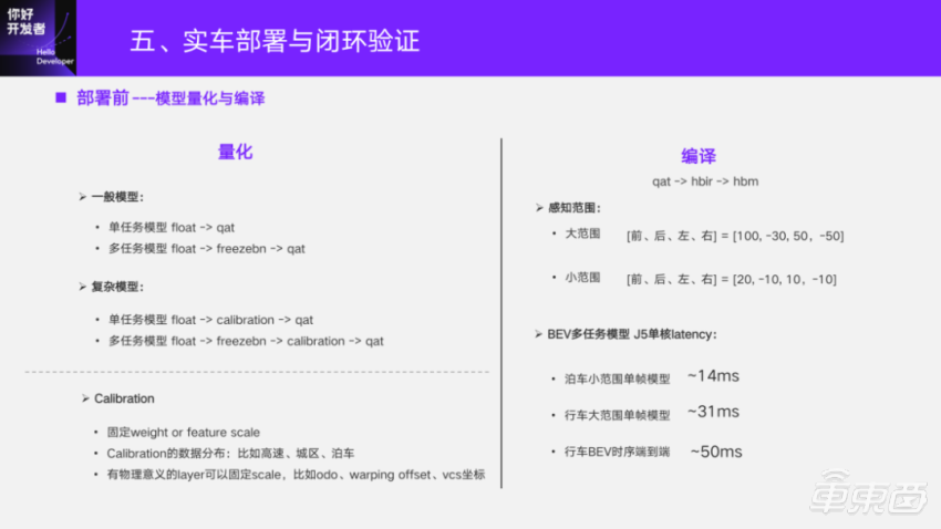
First of all, the model must be quantified and compiled before deployment. Professional quantitative processes and methods, we also arranged an open class to share later. I mainly look at this matter from the perspective of a user.

For the general model, such as CNN-based, we directly single-task float and directly train qat after training, which basically does not lose points. A freezebn will be added in the middle of multiple tasks, so that the counted bn can be applied to each task.

For complex models, a step calibration will be added. The key point here is calibration. Take our end-to-end model deployment as an example. As far as the single-task model is concerned, there are many drop points in the early end-to-end direct float training qat. After consulting my colleagues in the tool chain, I suggest that we do calibration. However, after calibration, it is found that although qat has been greatly improved, it still has a big gap with float. Colleagues in the tool chain suggest fixing the scale of weight or feature. Actually, it is more effective to fix the scale of the feature, but it does not completely solve the problem of qat output of the above tasks from end to end.

So what’s the problem? I also went to some pits. In fact, it is very simple to think about it now. We need to calculate the appropriate feature scale and select the appropriate data when doing calibration. For example, in the early stage, we used the data of urban scenes to estimate the feature scale of speed, and found that the qat index of the trained qat model in high-speed scenes was worse than that of the float. Later, through the tools of the tool chain, the model was analyzed layer by layer and it was found that the problems on the model could not be found. If there is nothing wrong with the model, it is a problem with the data. Finally, we use a high-speed data set. Because calibration itself has few training steps, it is necessary to select the quantity that can cover the perception and reach the upper and lower limits of the maximum and minimum values, so as to estimate a more suitable quantitative scale.

Despite this step, the problem of quantification has been greatly solved. However, the standard of tool chain is generally that the gap between qat and float cannot be greater than 1%. After these two steps, it still can’t reach this level. So what else went wrong? Later, it was also a groping, and it was found that many quantities of 3D perception on BEV were physically meaningful. The final conclusion is to fix the scale for some physical computing layers. Where does the fixed scale come from? For example, as mentioned earlier, the feature on the query index BEV has warping operation, and it has clear physical significance to calculate the two inputs of offset. When the model structure is determined, the maximum and minimum values of the meshgrid on BEV, as well as the maximum and minimum values of the query index, have been determined, so that the maximum and minimum values of the matrix can be calculated, and then the fixed scale can be calculated.

For example, taking odometry as the model input, the data of calibration may be collected at a medium speed, but the speed of the self-propelled vehicle may also change during the actual large-scale data training. Therefore, the maximum and minimum values can also be obtained for this physical quantity with clear rules. With a similar idea, check some numerical calculation layers with physical significance in the network and calculate the fixed scale. Through these operations, the qat problem of the end-to-end model is solved, and it is also a lot of experience. Let’s share it with you.

Quantization is compilation. Compilation means that the compiler directly converts the intermediate format hbir from qat, and finally gets the hbm format deployed on the real board. The specific details are also shared and introduced later. Here is mainly about the performance of BEV perception in actual deployment.

The large-scale BEV is the perception range of 100 forward, 30 backward and 50 left and right respectively, and the small-scale BEV is the perception range of 20 forward and 10 meters in the other three directions, so as to do the element perception on BEV. On the single core of Journey 5, such as a small parking area, the multi-task model of single core and single frame can reach more than 70fps; The wide range of driving can also reach more than 30fps. Even with end-to-end, the model directly output to trajectory prediction can reach more than 20fps, which is in the case of single core. There are two cores on Journey 5, and the frame rate can be further improved in model scheduling.

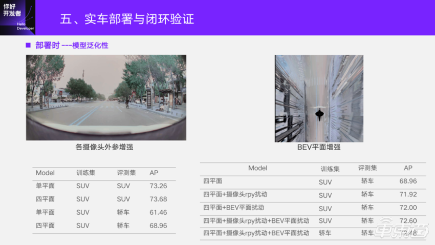
At the time of deployment, the generalization of the model is tested. Because the model of the customer’s car is different, the corresponding camera installation position and orientation may be different. Our BEV model, especially in the prototype development stage, has many customers who have been verified in the early stage, so a model can support the deployment of multiple models as much as possible, which requires a high generalization of the model. We have also explored a lot, and finally found that the four-plane spatial fusion method introduced earlier has laid a good foundation at the beginning. The example given here is that the training data are all collected by SUV, and the data of cars are used for evaluation. If it is a single plane, it has more than seven drop points compared with four planes.

On the basis of better generalization of the four planes, we will develop some enhancement strategies for training. There are two effective methods here: one is that the BEV model disturbs the image by the camera rpy in one stage, simulates the bumps in the process of vehicle driving, and enhances the image; In addition, it is assumed that the plane is in the place where the angle of view is converted, and then the plane enhancement is made on the plane where the camera leaves VCS, which is also assumed to be the disturbance of rpy.

With these two disturbance strategies, this performance (AP 72.60) can be achieved in the training and training of SUV models and measured in the car data set, which is similar to the performance of an adaptive car model that we have trained with nearly 1 million data collected in about 20 days. Therefore, these strategic feature ensure the generalization of our current BEV perception model in actual deployment.

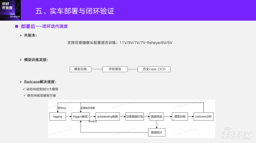
After deployment, the speed of closed-loop iteration of the model is tested. Especially in the verification stage of the previous prototype scheme, the demo closed-loop verification of different real vehicle installation and deployment is supported through a total version. For the BEV training framework, any camera configuration can be supported. For example, 11v/9v/7v, 7v may replace the 4v panoramic view with 4v fisheye, or any other multiple perspectives, all of which can participate in the model training. When deploying, compile according to the corresponding camera configuration, and then you can do the corresponding test.

The other is the training speed of the model, especially after the time series fusion. Without optimization, if a single frame is trained for 5 days and 10 frames are linear, it will bring 10 times the training time, which is definitely unacceptable. We definitely need to do optimization, and some students who have developed the framework specially guide us to do optimization. At present, the training speed has increased by 56% after optimization.

Specifically, at present, the multi-task release, multi-task with more than a dozen task heads, and the end-to-end training of time sequence can be completed within one week. The later evaluation or the case CICD of some historical data are all automated, thus ensuring the efficiency of the training and distribution step.

Another important factor, especially in the early stage of real vehicle testing, will feed back some non-working case-bad case data. How to use these data in training? There are generally two kinds of optimization for Badcase: one is to mine from the collected data, which is more conventional; The other is to be able to use the returned Badcase data directly.

For things like 2D perception, the link we did in mass production before was relatively mature. For BEV perception, the difference is to see how the model of the brush library comes from or how the data sent to the target comes from. For dynamics, a pure visual large model is used, which is not limited by on-board op and computational power. We have a big model team, and the pure visual BEV big model specially developed has also been used in the dynamic Badcase processing link to generate a pseudo GT to participate in the training. Static, a purely visual mapping scheme, can also send the base map to the standard, and has been deployed to the static perception Badcase link on BEV. In fact, after the deployment of the model, many of them are infrastructure problems. At present, the infrastructure of horizon’s perception of BEV is basically mature.

That’s all I shared today, mainly to convey a few meanings. First of all, based on the fact that Journey 5 can do many things, we have also done many things on it. For the BEV sensing scheme, we can see that we have a better baseline for reference and iteration, so the conclusion is relatively solid.

In addition, if some online students are developing based on Journey 5, or are about to develop based on Journey 5, when you encounter quantitative problems, don’t give up too early. Besides considering the model structure, analyze the data from the perspective of physical meaning and give it a suitable scale.

Finally, I wish everyone a smooth development, and my sharing today is over. Thank you!